• Word count: 1790
• Average reading time: 8 minutes and 56 seconds (based on 200 WPM)

Show me the code

When

Somwhere in the middle of 2015

Why

After having worked through Learn Python the Hard Way , Python Challenge and some tiny things for school projects I was up for a bigger challenge. I wanted to learn how to program something larger and utilize some of the things I learned through my studies. With image processing one is able to quickly see what something, for example a filter, is doing exactly. This 'feedback' is something I really enjoyed. Having decided upon a direction for a project (image procesing) I needed to figure out a project in this direction.

On top of this I had the desire to crawl second-hand car advertisement websites for aggregation. I noticed that some advertisements have good pictures of car license plates but lacked the license plate itself in the description. My idea was to enlarge the amount of license plates available in such a dataset so I'd have more detailed information of the cars in the advertisement. However, having no labelled training data I wanted to create a labelled training set by using a heuristic that can be used to create one for me instead of having to do it by hand.

I googled around for some implementations of ANPR and quickly stumbled upon this (pdf) paper. This paper had a very detailed approach for covering all the aspects involved. I decided to replicate this approach as an educative project.

Disclaimer: This project was started in my hey-day of programming (early 2015) and I have refractored the code significantly for better readability purposes. There is a lot of room for improvement and optimization in the code and in my final solution. Once again, the goal was to generate a large labelled training dataset from which I would manually drop false-positives, the machine learning algorithm that would be trained with the generated labelled training dataset would likely be far more robust.

How

Initially I started with matplotlib to open the image files and apply some filters to explore the functions but was quick to discover the OpenCV (cv2) and Scikit-image (skimage) libraries that added a whole lot more functions than matplotlib was able to provide.

Recreate the band clipping method:

The initial problem was just simply locating the license plate correctly. I started off with the method as provided by the author: Apply a vertical edge filter and sum the image on the X-axis and from this 2d representation extract the peaks. [page 7 & 8]

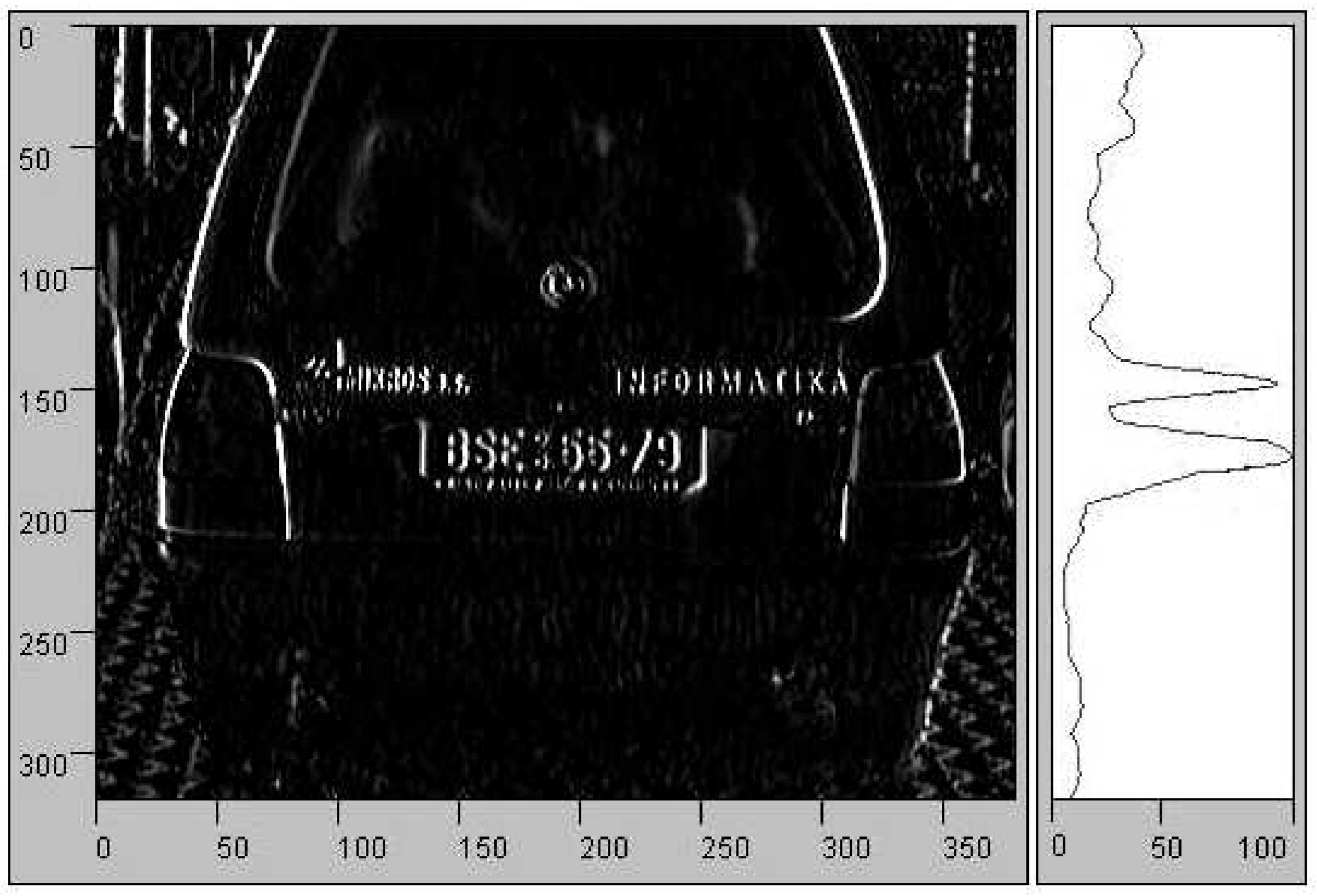
On first sight this seemed very promising but during my attempts to replicate I was quick to notice that this approach wasn't as good as I initially thought. Below this I have provided my attempt to replicate the above result. Do note that I have not applied a smoothing filter on the summed plot, this to illustrate how poor the performance was - a smoothing filter would've only made things worse. Also I have applied a general edge filter instead of a vertical edge filter as this seemed to capture the edges better than only a vertical edge filter.

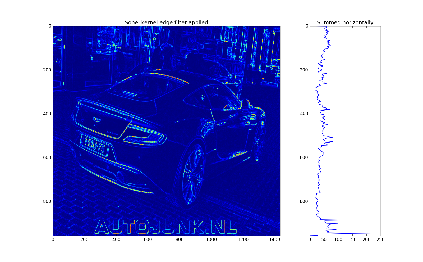
Obviously the characters at the bottom of the image skew the results but despite that no notable peaks around the y-axis position of the license plate seem to occur. Having used the double threshold approach as provided by the author [page 9-10]. I have attempted this approach with different kernels (Sobel & Feldman) and the different libraries, I had also implemented my own (extremely slow) implementation but neither of these approaches seemed to improve on the initial result.

Becoming stuck at this stage was a bit disheartening and in my desperation I started toying around with the examples that were on scikit-image and on OpenCV

The initial results of the scikit-image region labelling code looked promising and after tweaking the parameters for some time it started to look better and better.

My own approach

I dropped the paper for this stage and would come back later, if needed and viable, but decided that this approach was more fruitful and stable. To talk you through the approach I've made I will use this image as an example:

Label candidate characters

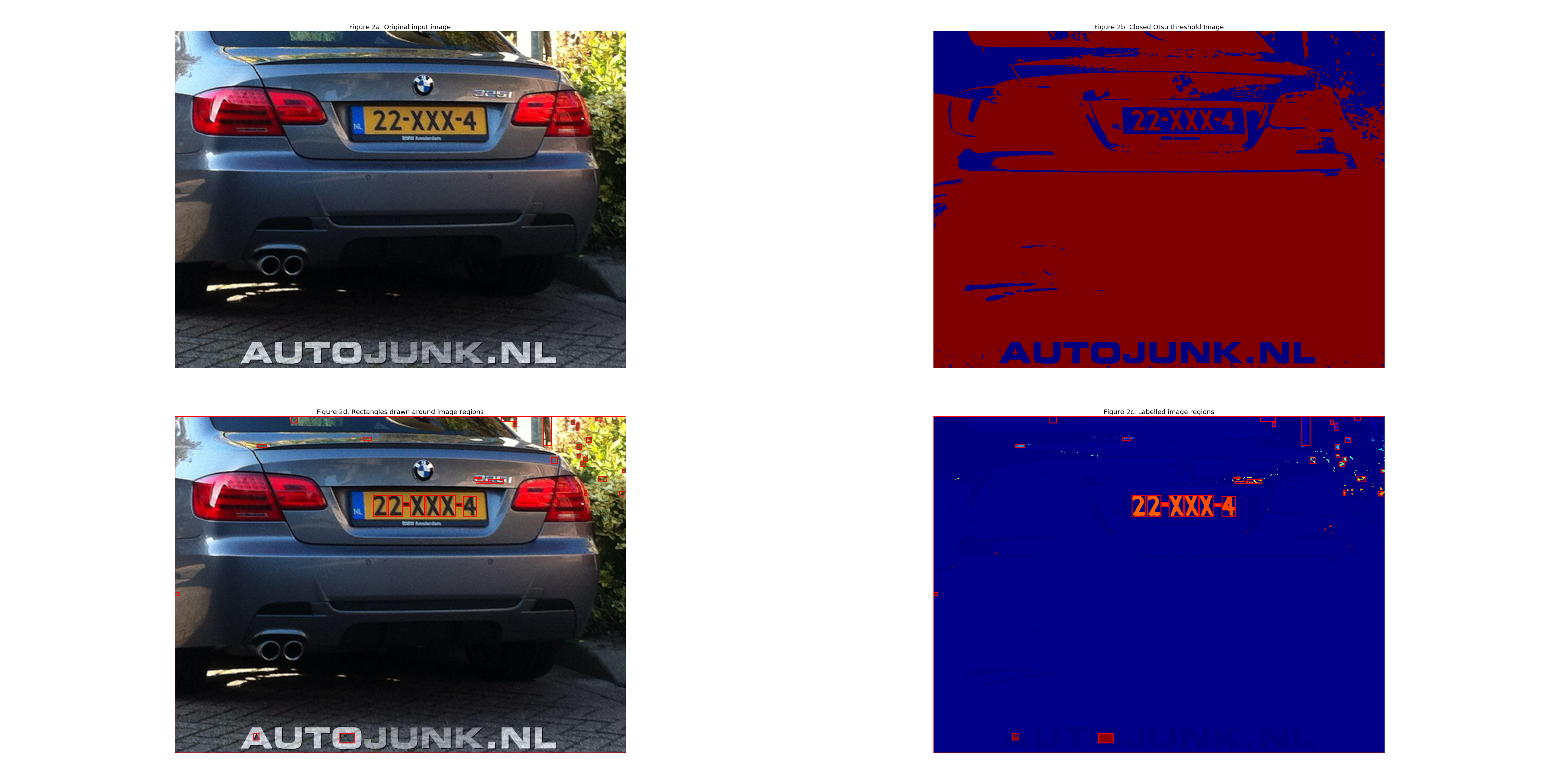
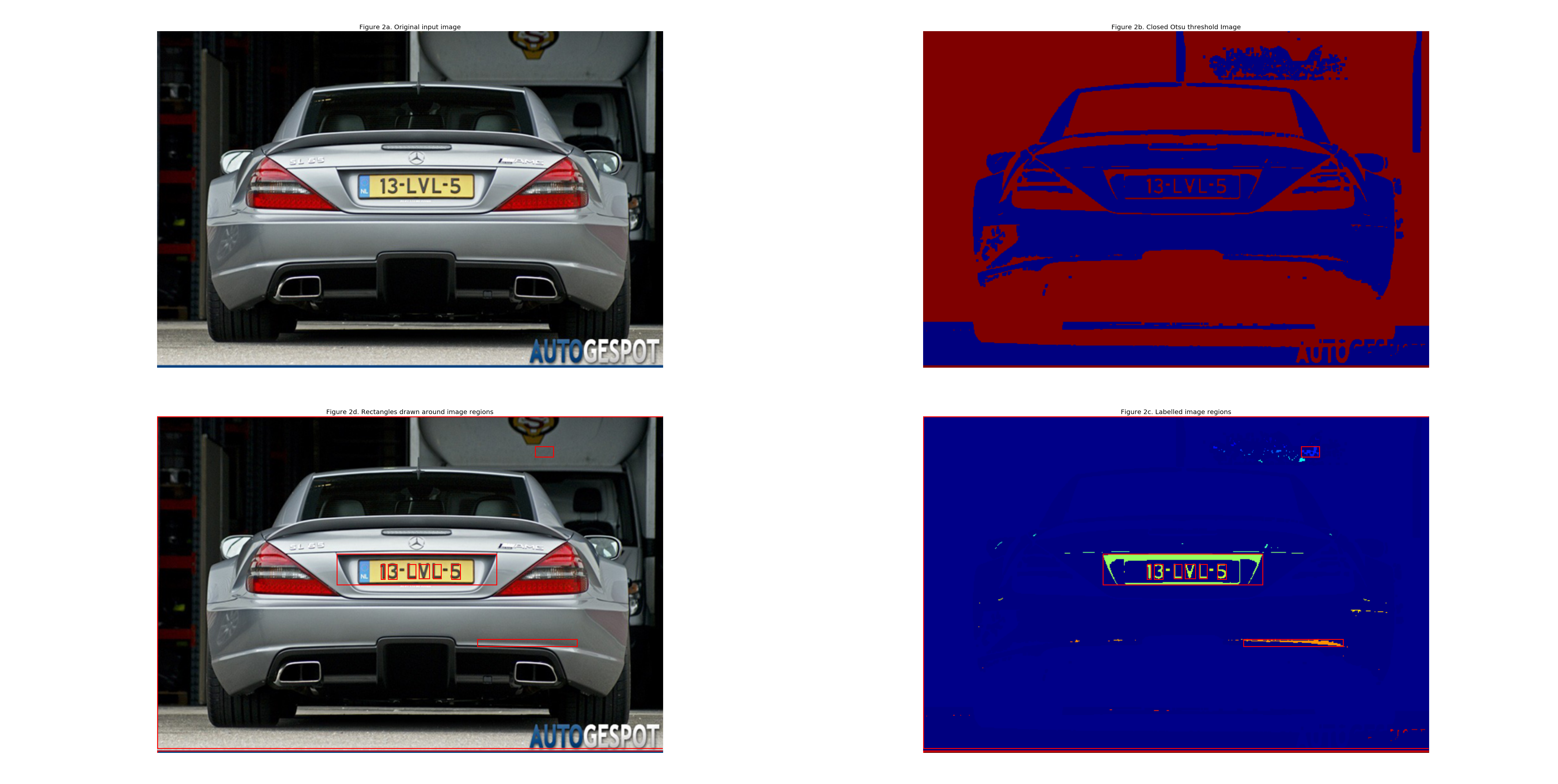
The image labelling is a simple process that can be covered in four steps as described in the documentation of the scikit-image example:

1. Apply automatic Otsu thresholding to generate a binary image (Figure 2b.)
2. Close small holes with binary closing (Figure 2c.)
3. Remove border artifacts (Figure 2c.)
4. Measure image regions to filter small objects. (Figure 2c & 2d)
5. Remove all not-standing rectangles (width > height) #License plate characters are taller than they're wide.

When applied these steps can be viewed in the image below:

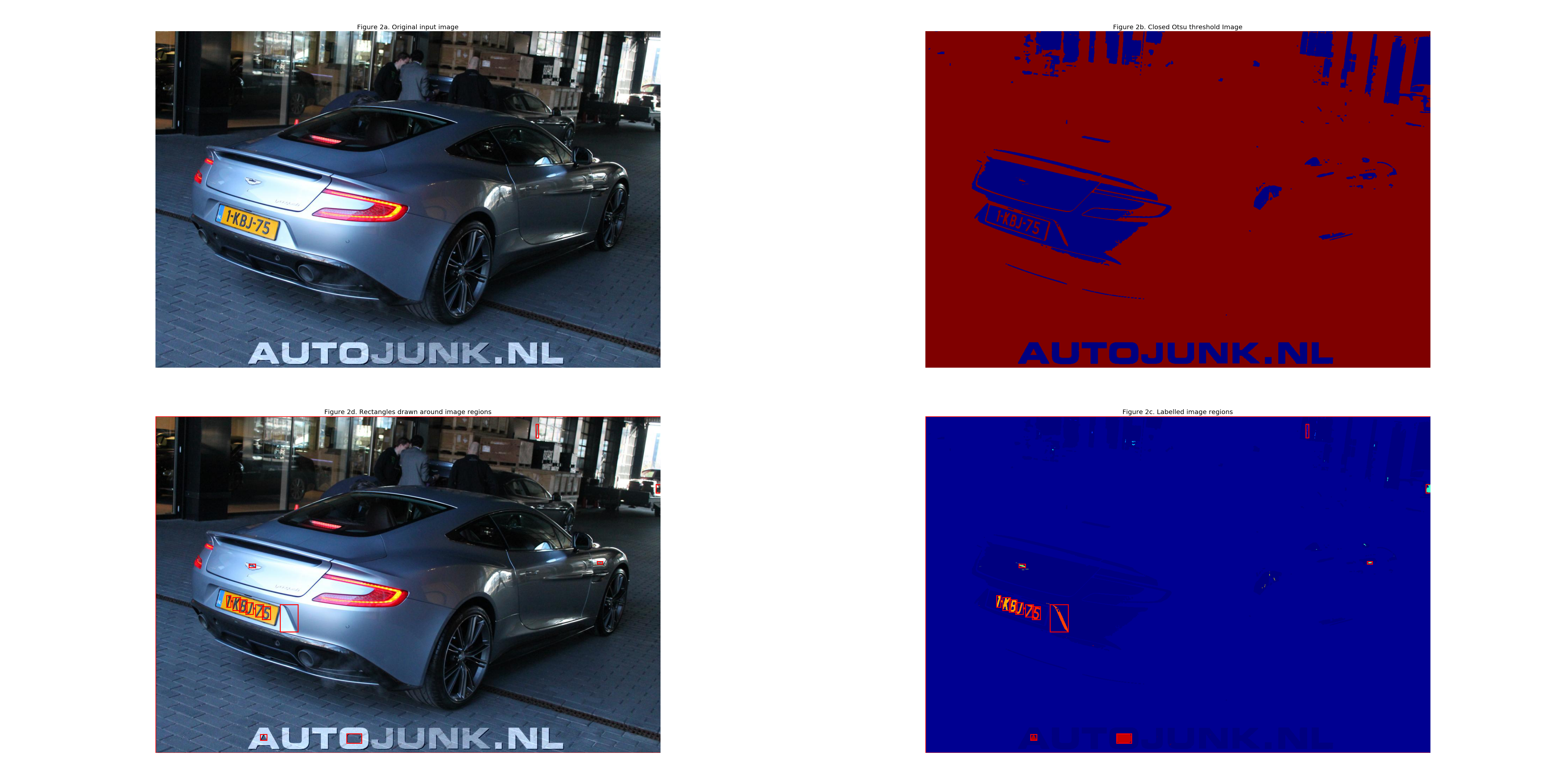
In this example almost only the characters of the license plate get detected bar some random regions in the image. In the image below a lot more regions get detected as well (top right corner in figure 2c & 2d)

Group the candidate characters

Due to the amount of regions it is difficult to figure out which ones belong to the license plate and which ones are to be interpreted as noise. To extract the correct regions I exploited one of the many characteristics of a license plate; characters are relatively close to each other. By enlarging the rectangles with \(width * 6\) and \(height * 2\) it becomes more clear which rectangles lie in each other's neighborhood.

This approach is best illustrated by the code itself:

def make_connected_graph_array(self, character_property_list):
    n = len(character_property_list)
    width_magnify = 3
    connected_matrix = np.zeros((n, n))
    counter_ar = np.zeros(n)
    for i in range(n):
        for j in range(n):
            if i == j: #No need to check a rectangle with itself
                continue
            target = character_property_list[i]
            original = character_property_list[j]

            target_height = target[3]            
            target_width = target[4] * width_magnify

            high_filter_pass = False
            width_filter_pass = False

            #target_Y1 + target_height >= original_Y0 >= target_Y0 - target_height
            if target[1][1] + target_height >= original[1][1] >= target[1][0] - target_height:
                high_filter_pass = True
            #target_Y1 + target_width >= original_X0 >= target_Y0 - target_width
            if target[1][3] + target_width >= original[1][2] >= target[1][3] - target_width:
                width_filter_pass = True

            #If either one of the original corners is within the range of the target rectangle than they overlap with each other
            if high_filter_pass and width_filter_pass:
                connected_matrix[i, j] = 1
                counter_ar[i] += 1

            #If a rectangle is inside another rectangle than remove it from the counter
            if target[1][0] > original[1][0] and target[1][1] < original[1][1] and target[1][2] > original[1][2] and target[1][3] < original[1][3]:
                counter_ar[i] -= 1
    return connected_matrix, counter_ar

For the image with the BMW 325i with license-plate 22-XXX-4 this array would look as follows:

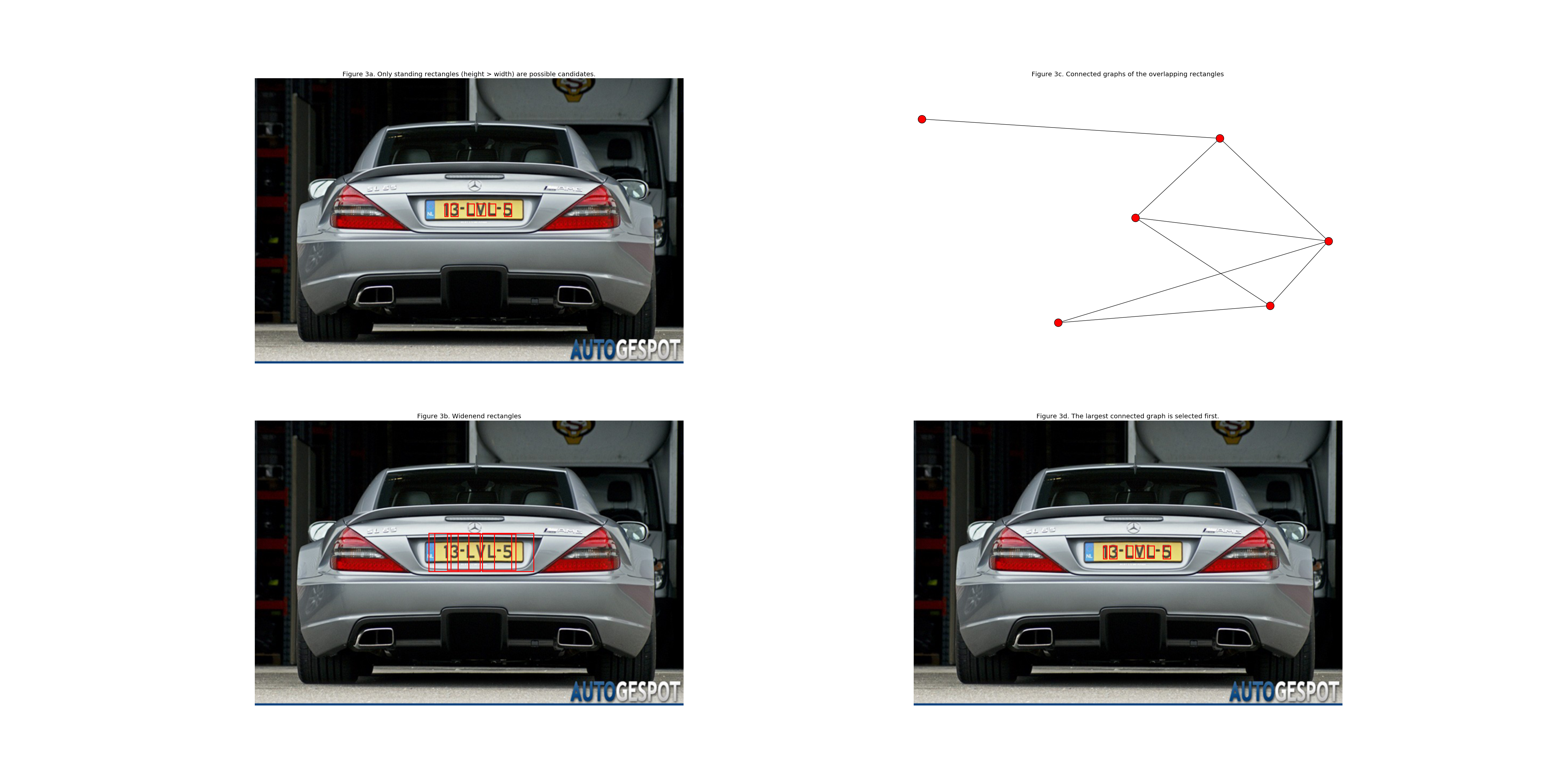
Extract the most likely group of characters

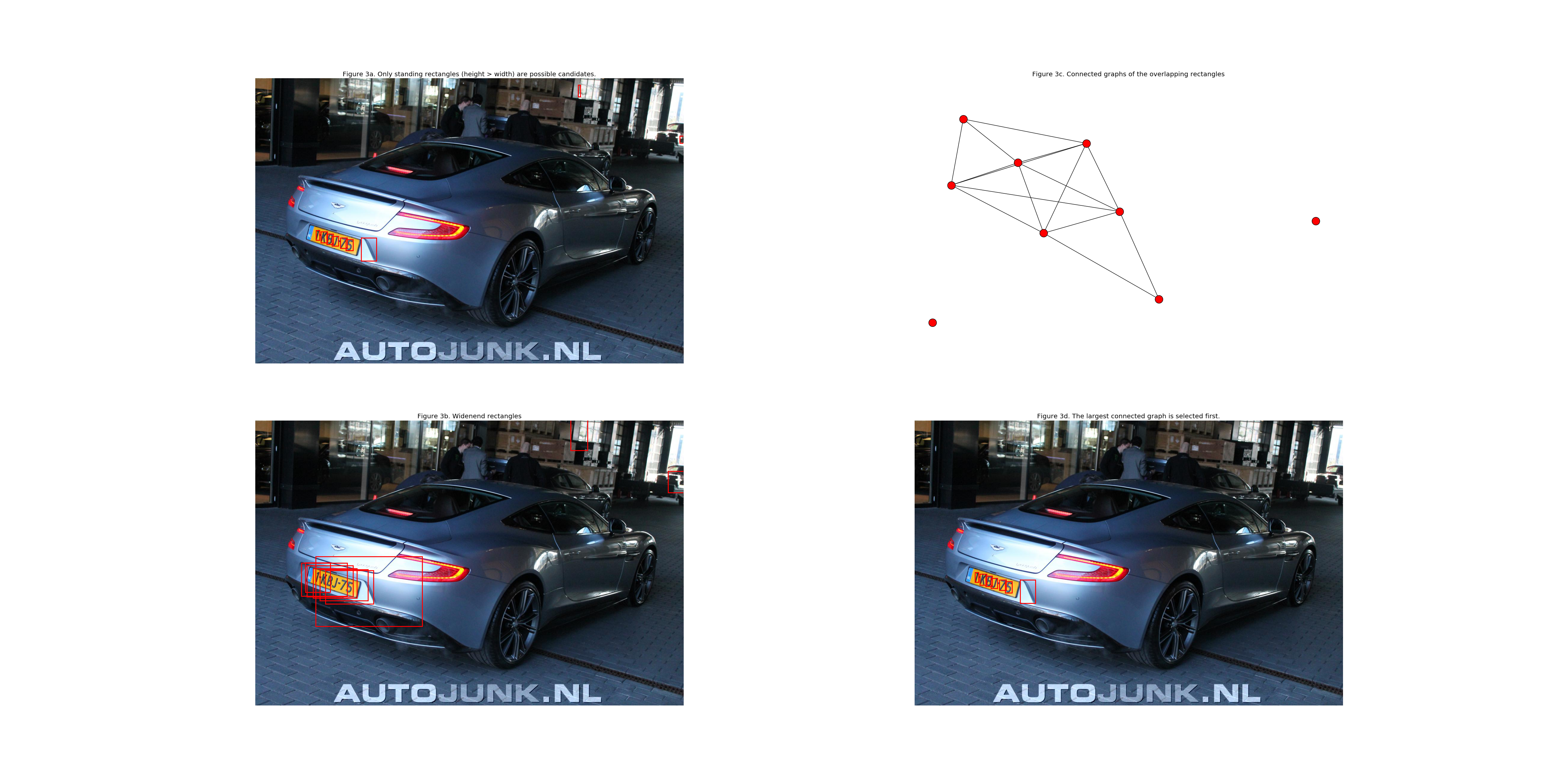
This array can be used to compute connected graphs. The connected graph with the largest amount of connections is used as a starting point; This is the most likely license plate. This proces can be summarized in the following steps:

1. Figure 3a: The original image with the original size rectangles
2. Figure 3b. Enlarged rectangles by making the rectangle 6 times as wide and 3 times as high
3. Figure 3c. The array is used to generate the connected graphs (the graph display is isomorphic)
4. Figure 3d. The connected graph with the largest amount of connections is selected and the remaining rectangles are plotted in their original size

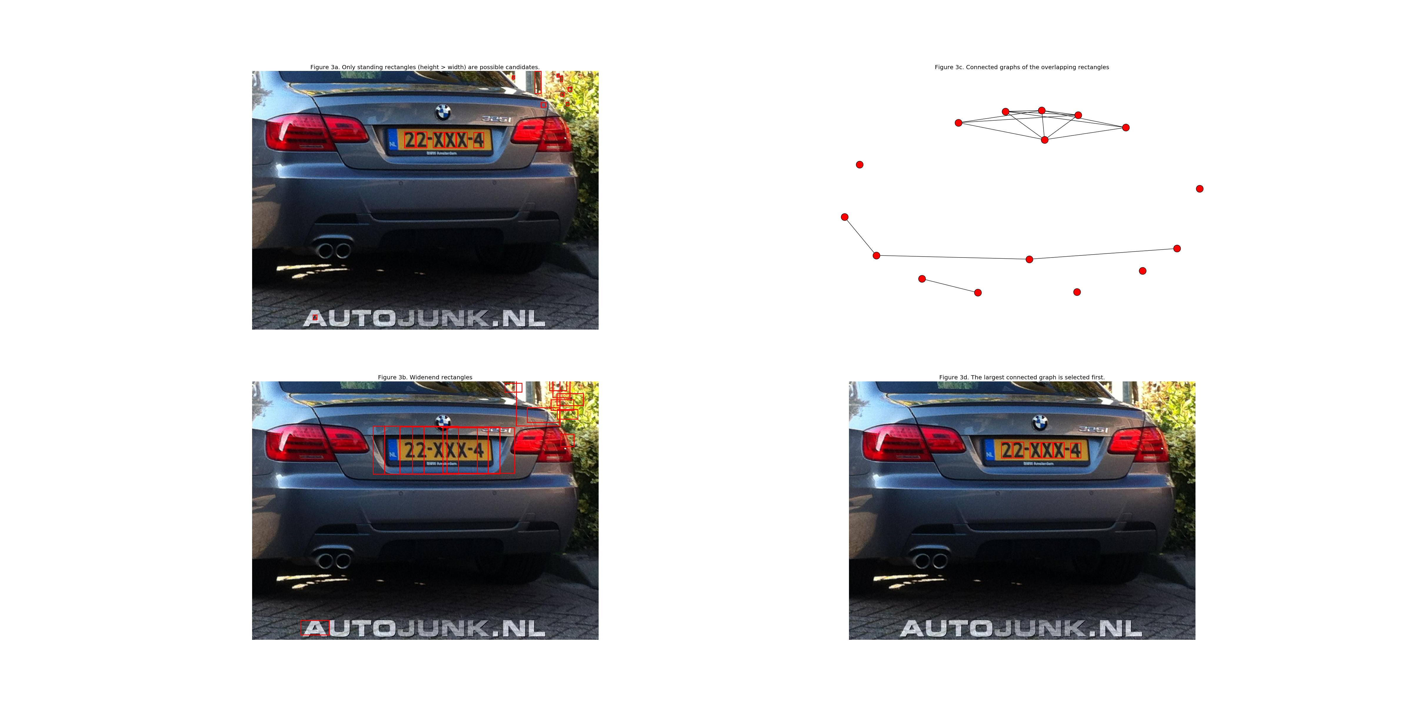
This worked quite allright in the above image but in the image of the Aston Martin a false positive character is selected as well, as can be seen below:

Filter false positives

To drop these from the selection one can use several characteristics of the license plate characters:

1. The surface area of the regions shouldn't vary too much.
2. The distance between characters and character groups:
   • The distance between characters right next to each other.
   • The space between character groups.
3. The grayscale pixel values of an image from a license plate character have an extreme distribution with most of their values being either completely white or completely black.

All these three characteristics can be combined to make it a more robust algorithm. However, for the sake of simplicity I choose to only exploit one of these characteristics: The distance between the selected rectangles.

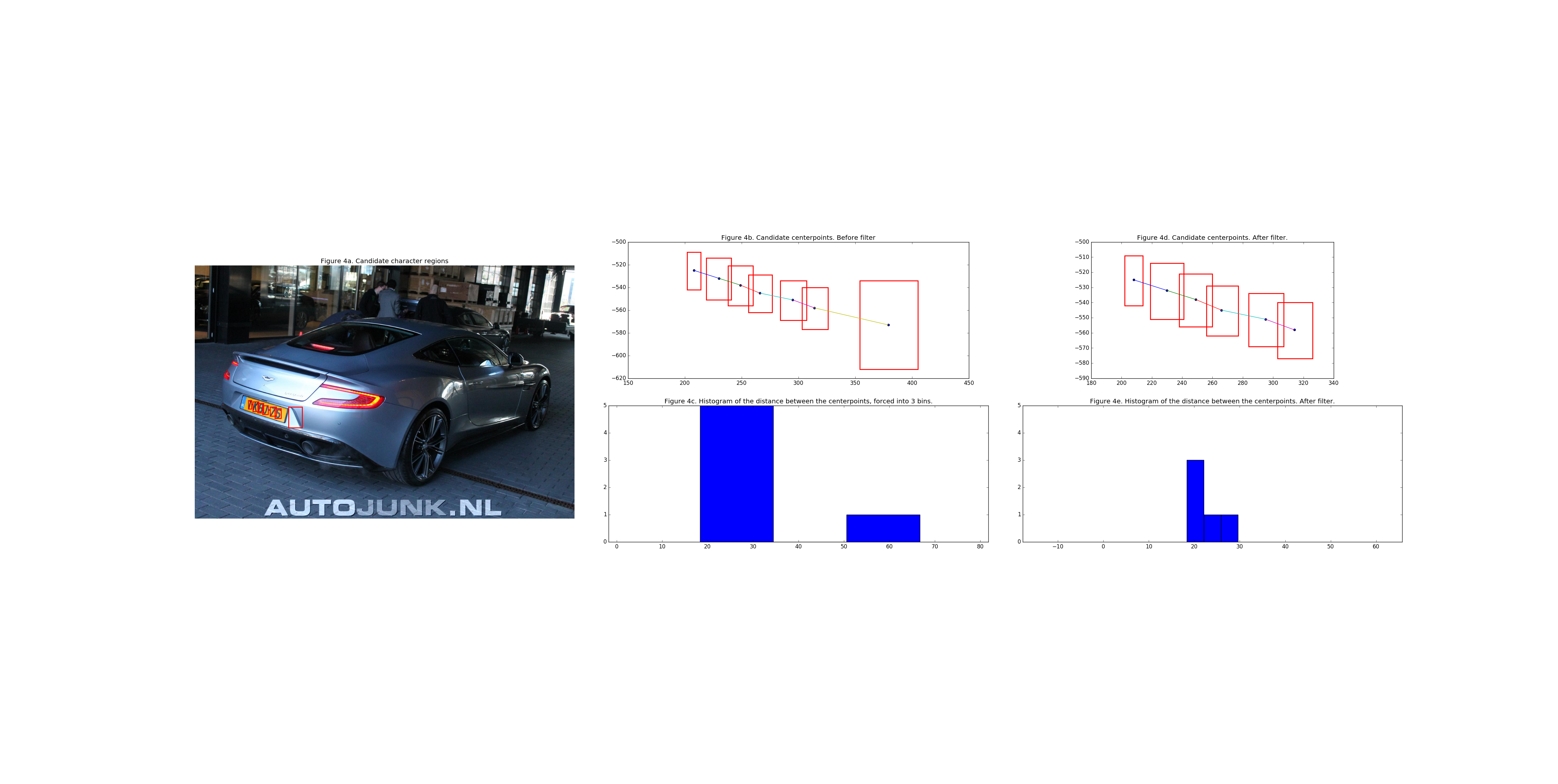
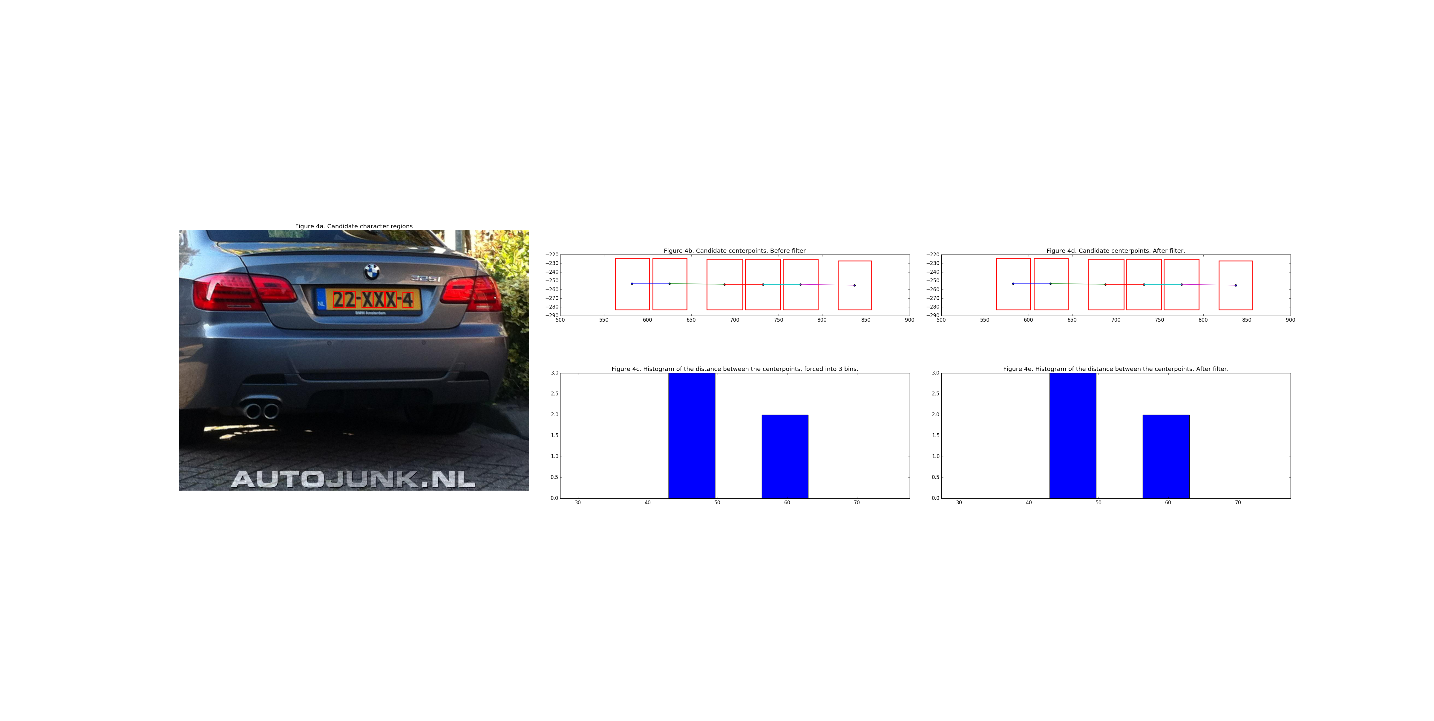
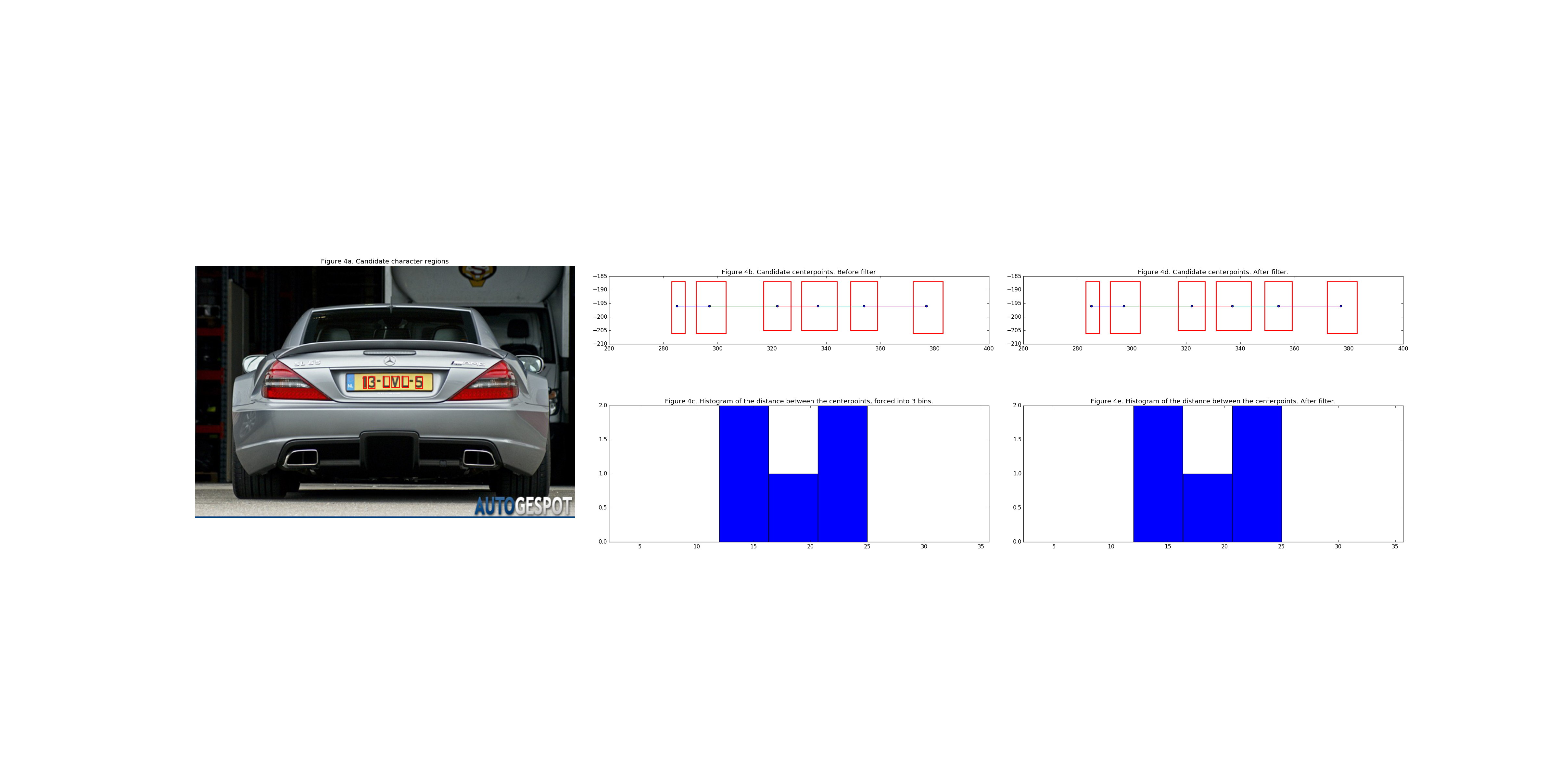
To exploit this characteristic a list of the distances between the centers of the rectangles is computed. 1. Compute the centers of the remaining rectangles 2. Compute the euclidean distance from center to center 3. Force this list of distances in a 3 bin histogram

In this 3-bin histogram the values themselves are not relevant, but merely the distribution of the bins. With a histogram of a verified license plate the histogram would ideally have a bin count distribution of: (3, 2, 0) or (3, 0, 2). Some deviations can be expected as license the rectangles are not perfectly aligned with the characters of a license plate. This is not a problem as long as the deviations in the bin size are relatively small and the total bin count is 5 (license plates have 6 characters so 5 distances between them)

However, when the difference in bin_counts are on the extreme end of the histogram scale, e.g.: (5, 0, 1) or (1, 0, 5) it is to be expected (gut-feel) that the singled out value is an outlier and can be dropped from the selection.

Below are two images illustrating the process of the bin count filter.

Clean and rotate the character images

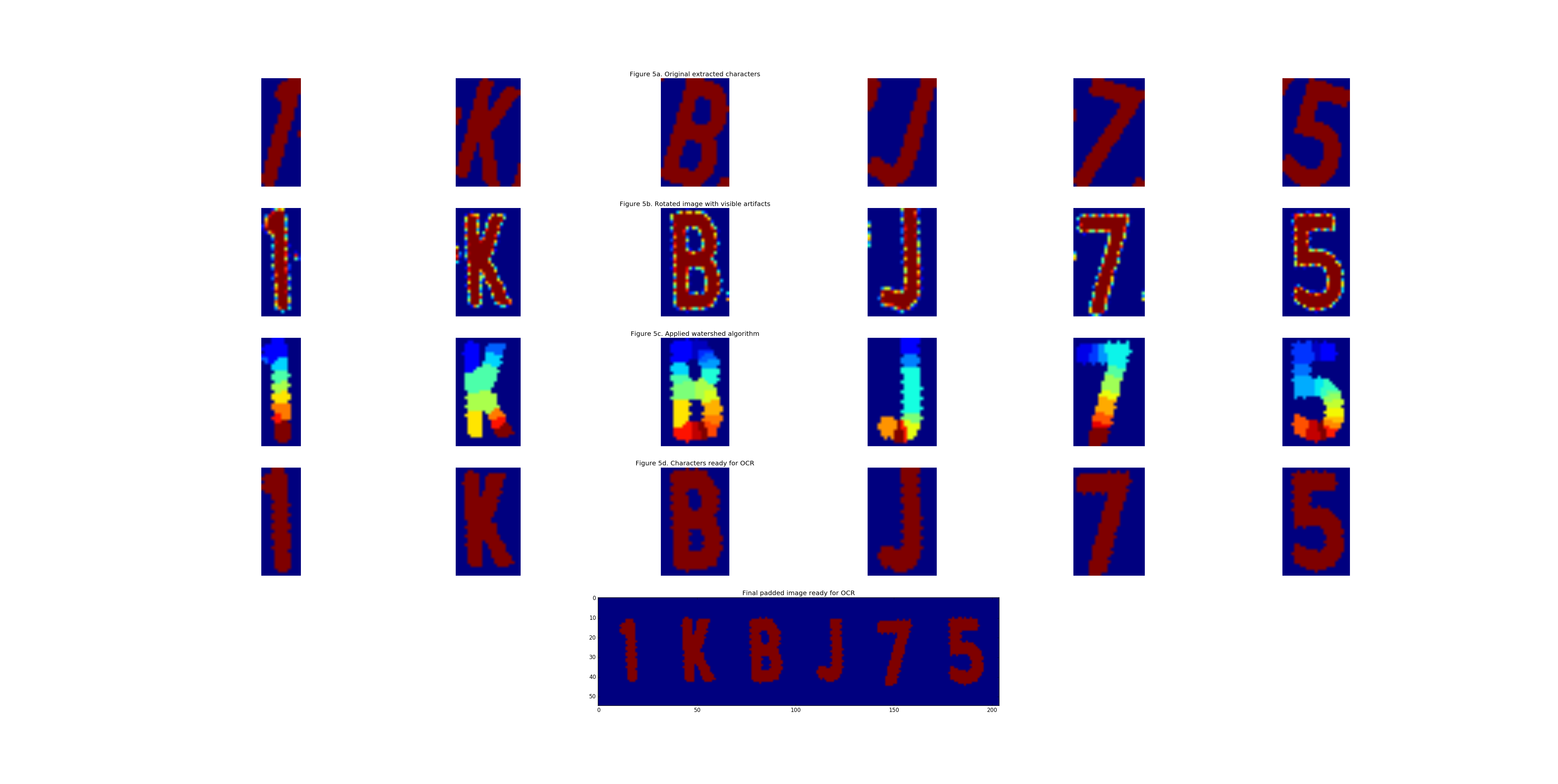
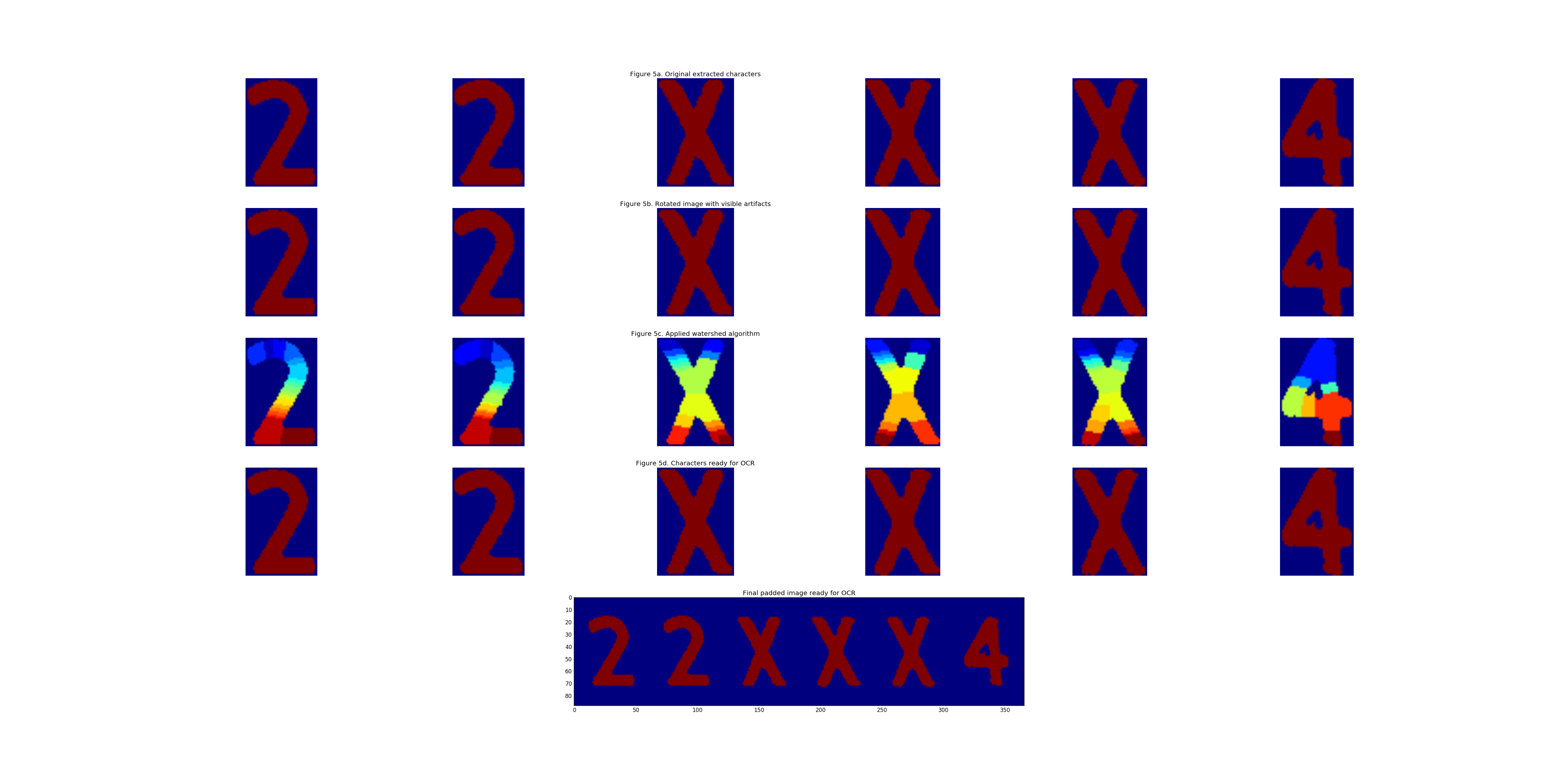
Now that it is highly likely the correct characters are extracted, the images need, if necessary, to be cleaned and rotated. This process is composed of the following steps:

1. Compute a linear regression line using Ordinary Least Squares and extract the coefficient. This coefficient is approximetaly the angle with which the characters need to be rotated. *This comes with extra artifacts which affects the quality significantly, thus the images are only rotated if the absolute value of the coefficient is more than 0.1
2. Rotate the images
3. Apply watershed algorithm to extract only the characters and remove noise.
4. Pad the images and concatenate them into a single image for character extraction.

This process is illustrated in the images below:

From this image it is quite easy to extract the characters, there are several approaches for this but the quickest way I found was using Pytesseract, a wrapper for Tesseract, the open-source OCR engine. Setting it up was quite easy and all that remained to do was to provide Tesseract with a white-list of avaiable characters.

Extract the characters

Applying tesseract on the above images results in the following output, respectively:

1KBJ75 ZZXXX4

As is visible the license plate of the BMW 325 was for a part not correctly identified, this is not too worrysome though. The goal was to generate a large training dataset. Ideally this would be filled with 100% correctly labelled data but I reckon that even partially correctly recognized & located license plates still provide value, though this is one of the many things that can be improved about this project.

Concluding, I'm happy with the result and might improve the project in the future but for now I'm okay with it as it is. Though if I were to improve this program in the future I'd improve it as follows:

1. If no candidate character group is found in the first try then:

   • iteratively adjust the kernel size of the closing algorithm
   • iteratively slice the sides of the image so the threshold of the otsu filter shifts.

2. If a candidate group is found improve the robustness by:

   • Utilizing more characteristics of the license plate.

3. If multiple candidate groups are found and the largest connected group appears to be a false positive then:

   • Iterate over the groups instead of breaking entirely.

Complete Pipe

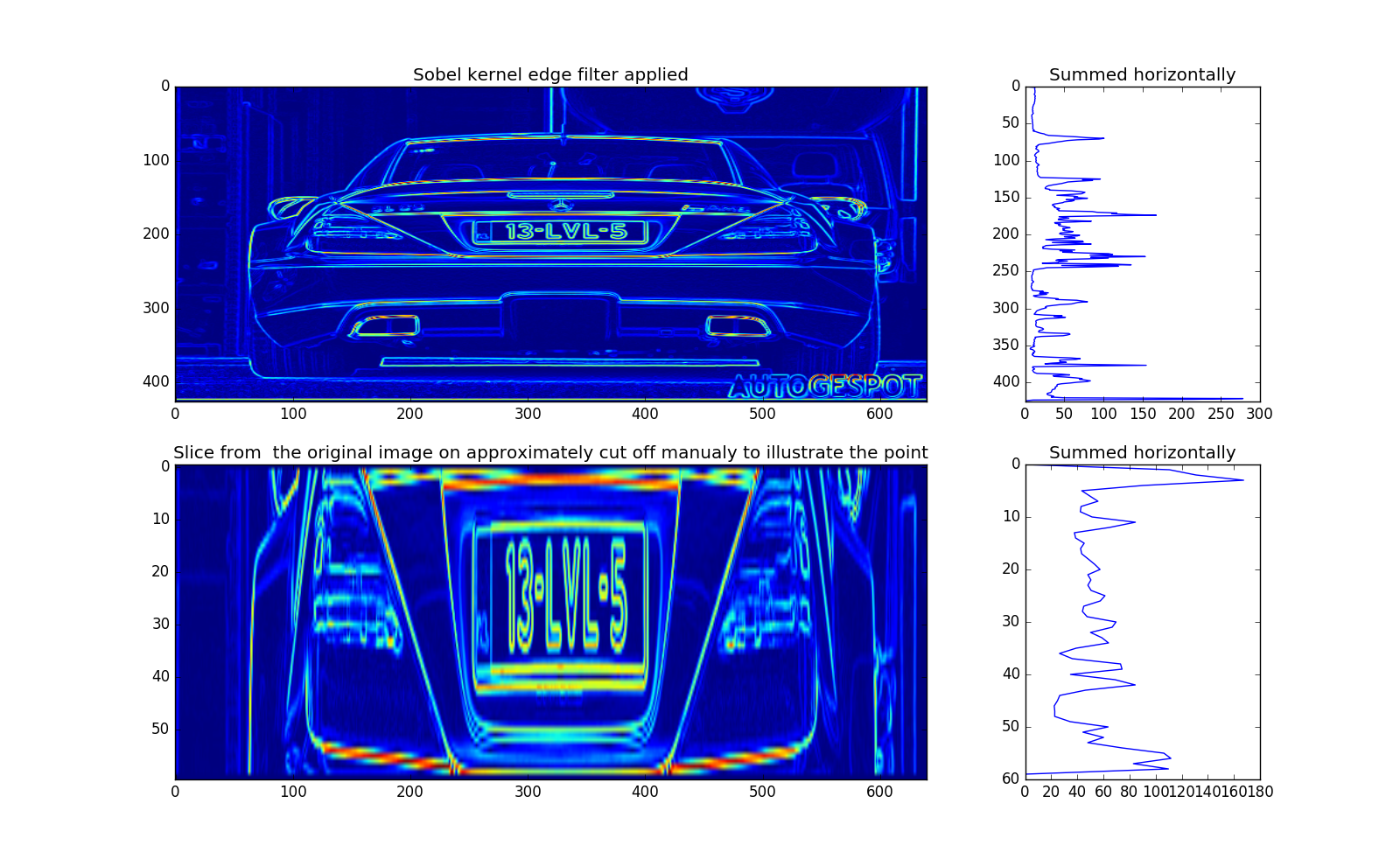
Finally I present the entire pipe of the algorithm on another image:

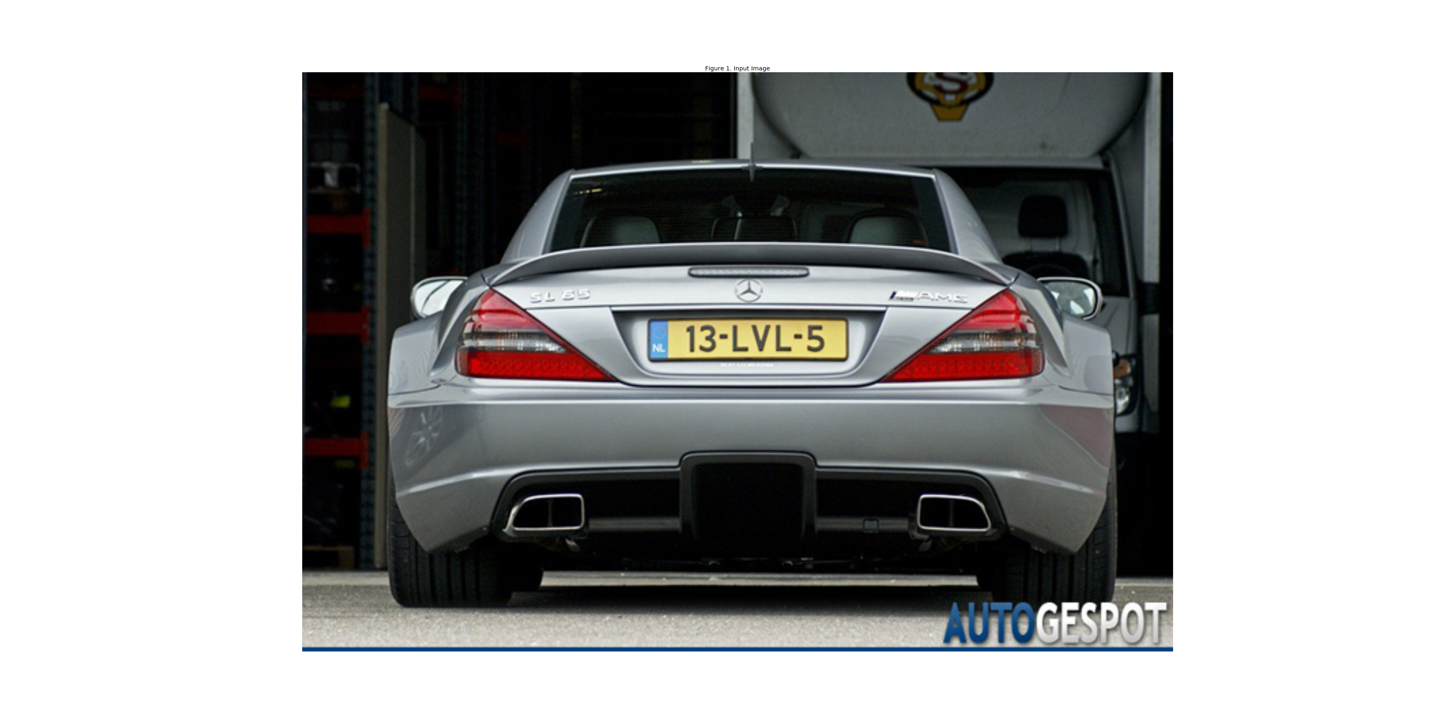
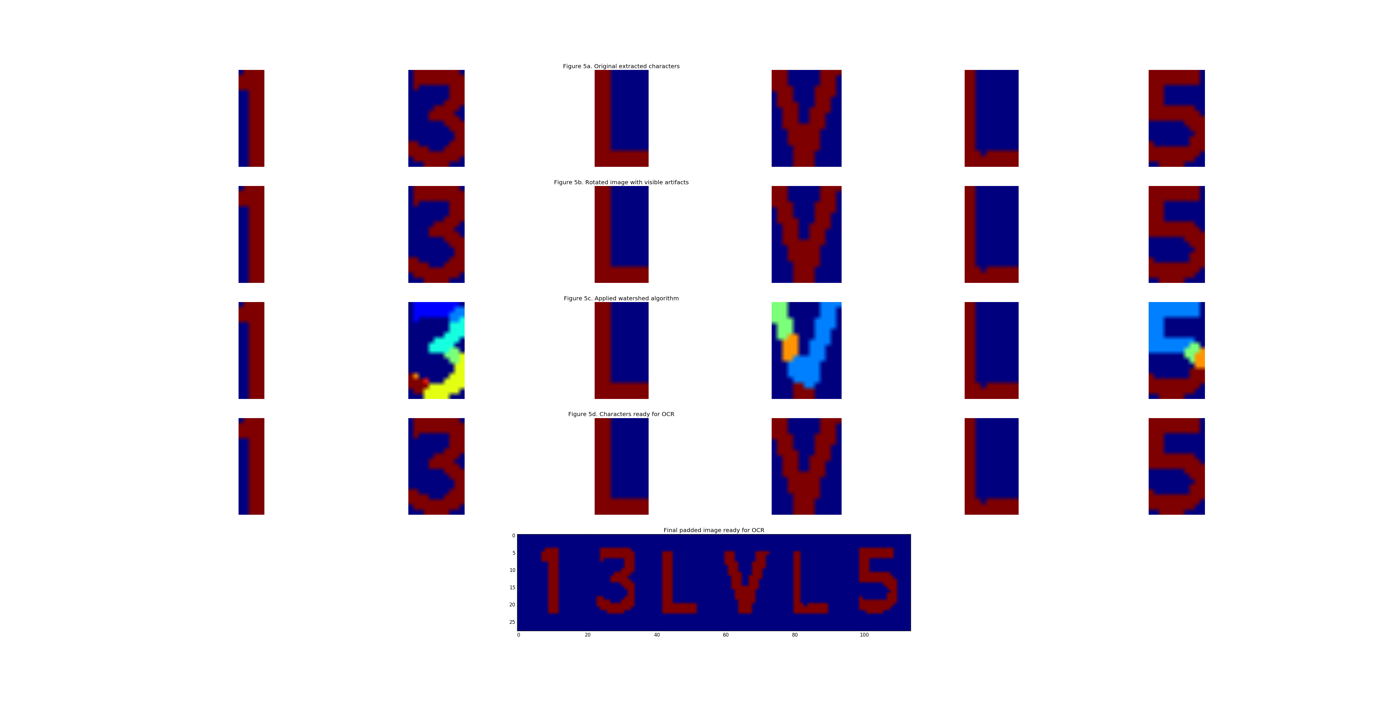
13LVL5